module Calculus.VisVerApp where

import Calculus

import Hatlab.Plot

Plotting with Hatlab

The brain likes seeing things. Let’s give it a good looking reward!

We’ll now make combined use of all of our nice functions. simplify, derive, integrate, eval, and show, all together: the most ambitious crossover event in history!

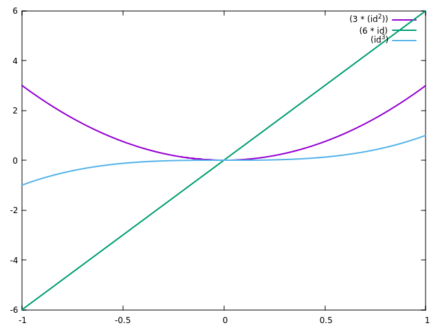
First, we create some function expressions ready to be shown and evaluated.

f  = Const 3 :* Id:^Const 2
f' = simplify (derive f)
_F = simplify (integrate f)

Then, we define a helper function to plot a list of function expressions with Hatlab.

plotFunExprs :: [FunExpr] -> IO ()
plotFunExprs = plot . fmap (\f -> Fun (eval f) (show f))

Now try it for yourself! Let’s see the fruits of our labour!

ghci> plotFunExprs [f, f', _F]

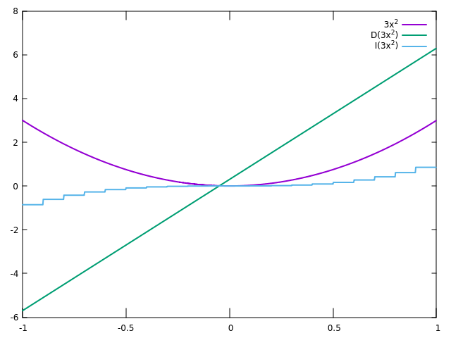
For fun, we can also plot the same functions but using our approximative functions for differentiation and integration

g x  = 3 * x^2
g' x = deriveApprox g 0.001 x
_G x = integrateApprox g 0.001 0 x

Then plot with

ghci> plot [Fun g "3x^2", Fun g' "D(3x^2)", Fun _G "I(3x^2)"]

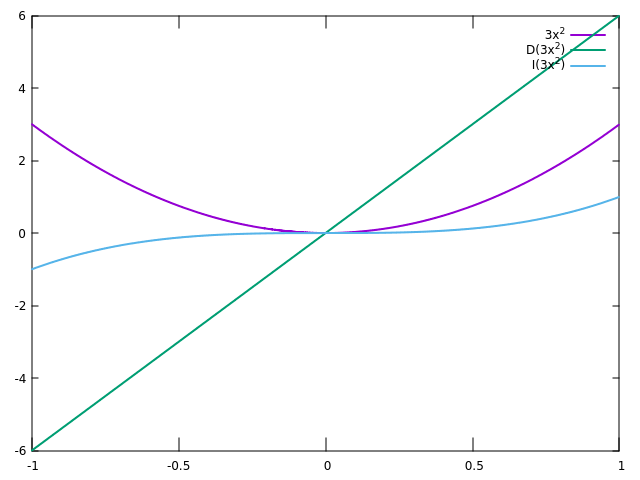
Waddaya know! They look identical! I guess it just goes to show that a good approximation is often good enough.

If we turn down the precision, we start to notice the errors

h x  = 3 * x^2
h' x = deriveApprox h 0.1 x
_H x = integrateApprox h 0.1 0 x

ghci> plot [Fun h "3x^2", Fun h' "D(3x^2)", Fun _H "I(3x^2)"]